Simulating 3D Gaussian random fields in Python
There is a lot of work studying Gaussian random fields (their definition, their statistical properties, and how to generate them) in the scientific literature. They are the underpinning of the study of cosmology and thus come up often in cosmological and astrophysical analyses. In this post, I’d like to go through an applied example of how to generate a 3D Gaussian random field (GRF) in Python with a user-specified power spectrum. In addition, I also demonstrate how to numerically compute the field’s Fourier coefficients in a volume-independent manner. See below for a few other nice references on GRFs:
Some preliminaries:
-
For non-astrophysicists, Mega-parsecs (Mpc) is a unit of distance, corresponding to \(10^6\) parsecs, where a parsec is roughly 3.3 lightyears.
-
Given a 3D field in real space \(\phi(x)\), its continuous Fourier transform is: \(\tilde{\phi}(k)(2\pi)^3 = \int \phi(x) e^{-ixk}dx\)
-
The power spectrum of a field is related to the square of its Fourier transform: \(P(k)\propto|\tilde{\phi}(k)|^2\)
-
The convolution theorem states that the multiplication of two functions is the same as the convolution of their Fourier transforms: \({\rm FT}(\phi\cdot\theta) = \tilde{\phi}*\tilde{\theta}\), where we sometimes call the Fourier representation of a function (e.g. \(\tilde{\phi}\)) a kernel.
1. Simulating GRFs
A Gaussian random field that is homogenous (statistically translation invariant) and isotropic (statistically rotation invariant) is defined uniquely by a power spectrum that is dependent only on the magnitude of the Fourier wavevector, and not it’s xyz components (i.e. depends only on \(|k|\) as opposed to \(\langle k_x,\ k_y,\ k_z\rangle\)). White Gaussian noise is a form of GRF that has power distributed equally on all size scales. We can therefore create a realization of a GRF by simply drawing independent samples from a Gaussian distribution. To then modify the distribution of power in the field, we can transform it into Fourier space, multiply by some function dependent on \(|k|\), and then transform back. Note that a GRF can also be defined by a Fourier series with random phases, thus generating a white noise real space field achieves this goal.
First we’ll generate a (real-valued) white noise 3D box.
First import Python modules
%matplotlib inline
import numpy as np
from scipy import stats, signal
import matplotlib, matplotlib.pyplot as plt
Generate a 3D box of white Gaussian noise
def sim_box(N, dL, seed=0):
    """
    N : number of grid cells per side
    dL : length of each grid cell
    """
    L = N * dL    # sidelength of box
    np.random.seed(seed)
    box = stats.norm.rvs(0, 1, N ** 3).reshape(N, N, N)
    return box

N = 400       # number of pixels per side
dL = 2        # sidelength of pixel (Mpc)

box = sim_box(N, dL, seed=0)
plt.imshow(box[0]); plt.colorbar()
Next let’s choose a power spectrum function. Let’s use a Gaussian tone at non-zero wavenumber. Note that the function we define here is the square-root of the power spectrum: \(P(k)^{1/2}\).
Power spectrum with a single tone in k-space
pk_func = lambda k: 1*np.exp(-.5*(k-.150)**2/.01**2)Now we need to generate the (k_x,k_y,k_z) wavenumbers for each voxel of box in Fourier space, then FFT the box, apply the pk shape and then transform back. Note that this is a FFT-and-multiply-and-iFFT process, so (based on the convolution theorem) we can also think of this as convolving the real space box with the power spectrum’s real space kernel.
Simulating a Gaussian random field with specified power spectrum
def sim_grf(box, dL):
    """
    box : 3D ndarray
    dL : pixel length
    """
    global pk
    N = len(box)

    # k spectrum of each axis
    k = np.fft.fftshift(np.fft.fftfreq(N, dL).astype(np.float32) * 2 * np.pi)

    # get 3D grid
    KX, KY, KZ = np.meshgrid(k, k, k, indexing='ij')

    # get K magnitude
    KMAG = (np.sqrt(KX**2 + KY**2 + KZ**2))

    # evaluate the pk function
    pk = pk_func(KMAG)

    # normalize by the noise equivalent bandwidth scaling (see below for explanation)
    pk /= np.sqrt(dL**3)

    # get the noise equivalent bandwidth of the pk function
    pk_NEB = np.sqrt(pk.size / (pk**2).sum())

    # note we use a symmetric FT convention here, which applies sqrt(L/2pi) for each axis for forward and backward
    bft = np.fft.ifft(np.fft.ifft(np.fft.ifft(
        box, axis=0, norm='ortho'), axis=1, norm='ortho'), axis=2, norm='ortho')
    bft = np.fft.ifftshift(bft)

    # apply the function
    bft *= pk

    # FFT back and take real (you can see imag is near-zero for yourself)
    grf = np.fft.fft(np.fft.fft(np.fft.fft(
        np.fft.fftshift(bft), axis=0, norm='ortho'), axis=1, norm='ortho'), axis=2, norm='ortho').real

    return grf, bft

grf, bft = sim_grf(box, dL)
And that’s basically it for simulating the Gaussian random field. Let’s look at the box before and after applying the power spectrum kernel:
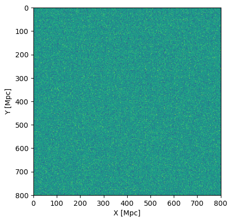
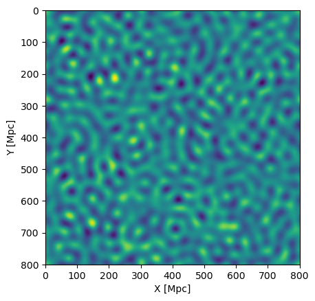
Figure 1 | Left: A white Gaussian noise field generated from `sim_box()` in real space. Right: The white noise box passed through a convolutional kernel defined by our chosen power spectrum function `pk_func()`.
We can also look at the 3D box in Fourier space, which visualizes the power spectrum function we chose.
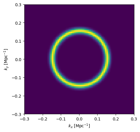
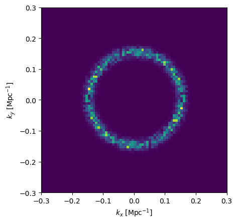
Figure 2 | Left: An analytic representation of the single-tone power spectrum function in Fourier k_x & k_y space (with k_x=k_y=0 at the center). Right: The absolute-value of the simulated GRF in Fourier k_x & k_y space. Note that its amplitude resembles the left plot but, because this is a single realization of the field, it has some amount of stochasticity.
Try keeping the box resolution the same (N) but increasing or decreasing the sidelength–notice that the ring in Fourier space increases in size. In other words, more of the white noise modes are either upweighted relative to the total size of the box. This means that the resulting grf will have more variance. We don’t want this! We want a GRF that has the same variance regardless of the box size or the voxel resolution (i.e. as if we are sampling the field as opposed to integrating it in voxel-sized windows). We can do this by normalizing the pk function by its equivalent bandwidth, which scales as \(dL^{3/2}\). This is key to estimating GRF power spectra that are the same regardless of the size of the box one simulates.
2. Estimating Fourier coefficients
Now let’s try to take the FFT of the box and compare against its power spectrum. Before, let’s discuss Fourier conventions.
We can choose to normalize the Fourier Transform integral on the forward pass, the inverse (backward) pass, or split the normalizing between both. This is given in numpy as norm='forward', 'backward', 'ortho' respectively. Recall in the preliminaries above there is a factor of \((2\pi)^3\) in the continuous forward Fourier transform. Our normalization convention amounts to whether we put this factor in the forward transform, the reverse transform, or whether we split it evenly between the two. Note that the 'ortho' convention ensures that the square integral of the modes is unity. For example:
Plotting discrete Fourier transform matrix inner products
plt.figure(figsize=(6, 5)); plt.tick_params(labelsize=16)
plt.plot((np.abs(np.fft.fft(np.eye(10), axis=1, norm='backward')) ** 2).sum(1), lw=3, label='backward')
plt.plot((np.abs(np.fft.fft(np.eye(10), axis=1, norm='ortho')) ** 2).sum(1), lw=3, label='ortho')
plt.plot((np.abs(np.fft.fft(np.eye(10), axis=1, norm='forward')) ** 2).sum(1), lw=3, label='forward')
plt.yscale('log'); plt.legend(fontsize=14); plt.title("Inner Product Values for n=10 DFT matrix")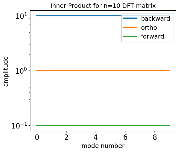
Figure 3 | Plotting the inner product of DFT matrices with different Fourier normalization conventions as a function of Fourier k bin.
The 'ortho' convention is nice for preserving symmetry between the forward and inverse calls, and for preserving the variance of the transformed field. Inspecting the modes, you can see that 'ortho' is simply \(e^{i2\pi k_mx_n}N^{-1/2}\) (where \(N\) is the number of x points): This property means that our Fourier transform coefficients will preserve amplitude regardless of the size of the box, which is what we want.
Okay, let’s take the 3D FFT of the grf using the ortho convention.
Compute 3D fft of a box with ortho-convention
def fft(grf, dL):
    """
    grf : 3D ndarray of gaussian random field box
    dL : pixel size (Mpc)
    """
    # compute fft and take abs
    gft = np.abs(np.fft.fftshift(
        np.fft.fft(np.fft.fft(np.fft.fft(grf,
                                         axis=2, norm='ortho'), axis=1, norm='ortho'), axis=0, norm='ortho')
    ))

    # multiply by sqrt(cell volume)
    gft *= np.sqrt(np.product(dL))

    return gft

gft = fft(grf, (dL, dL, dL))
One thing that the ortho convention leaves out is a factor of the voxel volume when taking the FFT, which acts as a normalizing factor. This volume is defined as \(V_p = \Delta L_x\ \Delta L_y\ \Delta L_z\), which we multiply in by ourselves in the fft() function. Note that it takes the form \(\Delta L^{3/2}\) because the power spectrum is related to the square of the field.
Now that we have our Gaussian random field as a 3D box in Fourier space, we want to form its power spectrum, which is simply the square of the Fourier coefficients.
\begin{align} \hat{P}(k_x, k_y, k_z) = |\tilde{\phi}(k_x, k_y, k_z)|^2 \end{align}
where \(\hat{P}(k)\) denotes an estimate of the true underlying power spectrum \(P(k)\).
With the 3D power spectrum in hand, we’d like to compress it down to a 1D power spectrum. This averages out inherent stochasticity in our random draw of the field, and is a permissible operation because, as we said before, the homogenous and isotropic GRF is defined only by the absolute magnitude of the Fourier wavenumber, not its separate components \(k_x,\ k_y,\ k_z\). Thus we can bin our 3D power spectrum in spherical annuli and average them up!
Bin the 3D power spectrum down to 1D
def gft_bin(gft, N, dL, K):
    """
    gft : 3d ndarray of GRF in Fourier space
    N : number of pixels per side length
    dL : length of pixel
    K : ndarray, the desired k-sampling of the 1D power spectrum, in units Mpc^-1
    """
    kx = np.fft.fftshift(np.fft.fftfreq(N[0], dL[0])*2*np.pi).astype(np.float32)
    ky = np.fft.fftshift(np.fft.fftfreq(N[1], dL[1])*2*np.pi).astype(np.float32)
    kz = np.fft.fftshift(np.fft.fftfreq(N[2], dL[2])*2*np.pi).astype(np.float32)
    KX, KY, KZ = np.meshgrid(kx, ky, kz, indexing='ij')
    KM = np.sqrt(KX ** 2 + KY ** 2 + KZ ** 2)

    Kdiff = np.diff(K)[0]
    BINS = []
    NUM, PK = np.zeros(len(K)), np.zeros(len(K))
    for i, k in enumerate(K):
        match = np.where((KM > k-Kdiff/2) & (KM <= k+Kdiff/2))
        BINS.append(gft[match])
        NUM[i] = len(BINS[-1])
        PK[i] = np.mean(BINS[-1] ** 2)

    return PK, NUM, BINS

# select 1D k sampling
K = np.arange(0.0, 0.40, 0.005)

# bin the gft box
PK, NUM, BINS = gft_bin(gft, (N, N, N), (dL, dL, dL), K)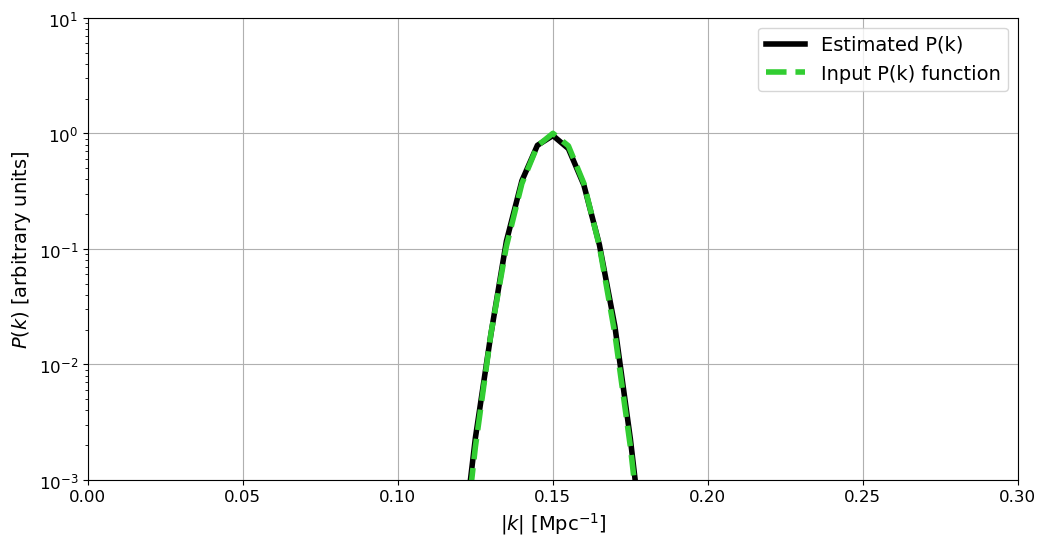
Figure 4 | Plotting the estimated and binned power spectrum (black) against the input analytic function used for drawing the field (green).
Figure 4 shows the resulting estimated power spectrum from our GRF (black), compared against our input analytic power spectrum curve (green), showing good agreement between the two! Next, we will repeat this process while varying the size of the box and of the voxel volume to ensure we can still correctly estimate the power spectrum of the field.
3. Ensuring invariance with respect to box size
Now we want to ensure that the computed power spectrum of the field is indeed the same regardless of the size of the box we use to take the FFT and the spacing of the voxels (i.e. the voxel volume). Also related is the application of any tapering (aka windowing or apodization) functions applied to the real space box before taking the Fourier transform (which modulates the effective volume of the box).
Different sized boxes – first let’s look at running our GRF power spectrum code through the same simulated box, but now having changed the size of the box and/or the volume of the voxels. We will look at three cases
- Take a quadrant of the original box (i.e. smaller box size)
- Take every other voxel along x,y,z (i.e. making the voxels eight times as large)
- A mix of both of these
Compute FFT(GRF) for different sized boxes
# smaller box but the same voxel size
gft = fft(grf[:300, :300, :300], (dL, dL, dL))
PK_1, NUM, BINS = gft_bin(gft, (300, 300, 300), (dL, dL, dL), K)

# stride the box so the effective voxel sidelength doubles
gft = fft(grf[::2, ::2, ::2], (dL*2, dL*2, dL*2))
PK_2, NUM, BINS = gft_bin(gft, (N//2, N//2, N//2), (dL*2, dL*2, dL*2), K)

# a mix of both
gft = fft(grf[:300, ::2, :300], (dL, dL*2, dL))
PK_3, NUM, BINS = gft_bin(gft, (300, N//2, 300), (dL, dL*2, dL), K)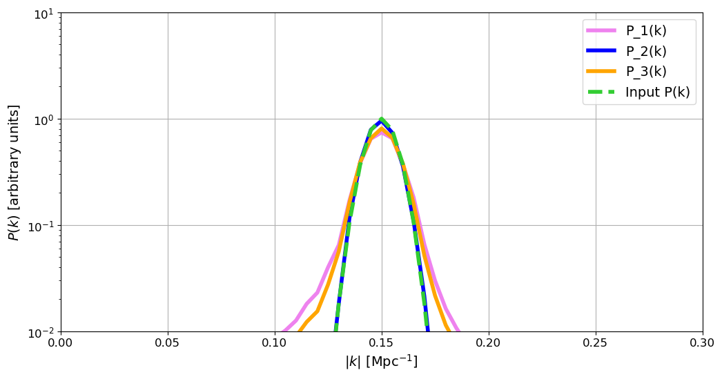
Figure 5 | Power spectra for the different boxes (1, 2, & 3), compared against the original input analytic P(k). We see that (to first order), the power spectra all agree with each other. Note that the pink and orange curves are slightly modulated by the fact that the smaller box leads to poorer k-space resolution, which acts as an effective rolling average of the field in k-space, thus slightly lowering and widening the peak. We will see this same effect below but with a slightly different cause.
Figure 5 shows that the power spectra of the various boxes all agree with each other (to first order, see the caption), thus our goal of ensuring volume and voxel-size-independent measurements of the power spectrum has been achieved. Next we will look at another, slightly more complicated way of altering the effective size of the box via a tapering function, which will also help expalain the minor discrepancies seen in Figure 5.
Tapering (aka windowing or apodization) functions–often in specral analysis we apply what’s called a tapering (or windowing, or apodization) function to the signal before taking its Fourier transform. This is needed when working with real data that is often not strictly periodic, which violates the key assumptions of the discrete Fourier transform and creates the well-known “ringing” phenomenon in Fourier space. The application of a windowing function makes our non-periodic signal more closely obey these assumptions, reducing the spectral leakage observed in Fourier space (in signal processing speak, we say that the signal sidelobes are reduced). The trade-off is a wider “main lobe” (the width of the main signal feature in Fourier space). Another way of thinking about a tapering or windowing function is that you are reducing the “effective size” of the box in a smooth way, rather than the hard cutoff we used above by looking at just a chunk of the box. This means we need to take this reduced volume into account, which can be done by computing the effective bandwidth of the tapering function, shown below.
Compute equivalent bandwidth for Blackman-Harris tapering function
# generate tapers for x,y,z axis
taper1 = signal.windows.blackmanharris(N)[:, None, None]
taper2 = signal.windows.blackmanharris(N)[None, :, None]
taper3 = signal.windows.blackmanharris(N)[None, None, :]

# compute noise equivalent bandwidth and normalize the taper
NEB1 = np.sqrt(taper1.size / (taper1 ** 2).sum())
NEB2 = np.sqrt(taper2.size / (taper2 ** 2).sum())
NEB3 = np.sqrt(taper3.size / (taper3 ** 2).sum())

taper1 *= NEB1
taper2 *= NEB2
taper3 *= NEB3


# apply taper to box and compute its grf and PK
gft = fft(grf * taper1 * taper2 * taper3, (dL, dL, dL))
PK, NUM, BINS = gft_bin(gft, (N, N, N), (dL, dL, dL), K)
Thus we have created normalized taper functions that account for the smaller box volume induced by the tapering. We show what the tapering does to the simulated GRF box below in Figure 6.
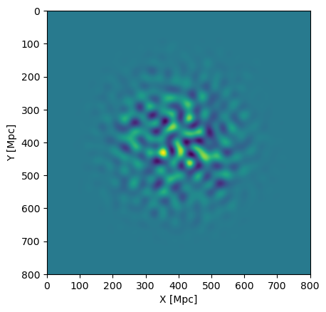
Figure 6 | The simulated single-tone Gaussian random field, tapered by a Blackman-Harris function along the x,y,z directions. The tapering downweights the edges of the cube, which reduces the effective volume of the box.
The effect this has on the power spectrum can be derived by computing the window function of the operation–not to be confused with the tapering function defined above! The window function is a convolutional kernel that acts on the power spectrum in k-space and accounts for the effect of a specific operation. Using the convolution theorem, we can see that multiplying the field by a taper in real space is the same as convolving the field’s Fourier transform by the taper’s effective kernel function, which happens to be the window function we are looking for. We can see how this makes our power spectra agree even better when we take this factor into account.
Compute the window function for a BlackmanHarris tapering function
# generate an approximate window function from one of the tapering functions
tfft = abs(np.fft.fft(taper1.squeeze())) ** 2
tk = np.fft.fftfreq(N, dL) * 2 * np.pi
from scipy.interpolate import interp1d
kernel = interp1d(tk, tfft, kind='cubic')(np.fft.fftshift(K - .2))
kernel /= kernel.sum()
kernel = np.repeat(kernel[None, :], len(kernel), axis=0)
for i in range(len(kernel)):
    kernel[i] = np.roll(kernel[i], i)
Now that we have our appropriate window functions (in k-space), we can go ahead and convolve it against the analytic input curve to get an “expected power spectrum” function. The result is shown below (we show the plotting script here to demonstrate how to do the window function convolution):
Plot the measured and expected GRF power spectra
plt.figure(figsize=(12, 5)); plt.tick_params(labelsize=12)
plt.plot(K, PK, lw=4, c='k', label='Estimated P(k)')
plt.plot(K, pk_func(K)**2, lw=4, ls='--', c='limegreen', label='Input P(k)')
plt.plot(K, kernel @ (pk_func(K)**2), lw=3, ls='--', c='r', label='W * Input P(k)')
plt.yscale('log')
plt.ylim(1e-3, 1e1); plt.xlim(0, 0.3); plt.grid()
plt.legend(fontsize=14)
plt.xlabel(r'$|k|$ [Mpc$^{-1}$]', fontsize=14); plt.ylabel(r'$P(k)$ [arbitrary units]', fontsize=14)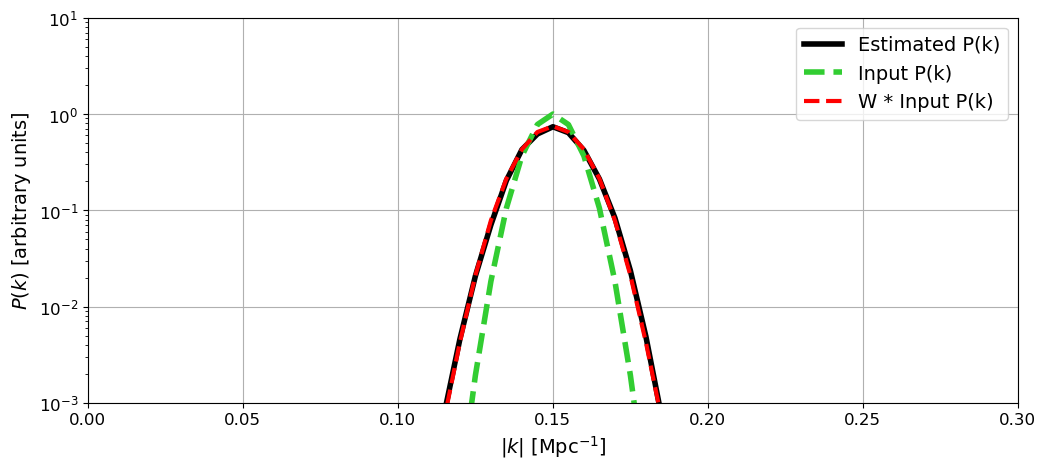
Figure 7 | The estimated power spectra from the tapered box (black), the input analytic power spectrum (green) and the input analytic function convolved by the taper's window function (red). The appropriate comparison is not black to green but black to red, which we can see is in good agreement.
Now that we have our window function we are prepared to make a faithful comparison of the estimated power spectra (black) and our “ground truth” for what it should look like (red). We can now see that this comparison is in much better agreement, showing the expected reduction in amplitude and widening of the main-lobe of the signal in k-space. The same kind of window function could be derived for the power spectra shown in Figure 5, improving the agreement between the measured and expected power spectrum.
As a side-note: what kind of window function should we expect in the case of taking a quadrant of the box, as we did in Figure 5? Taking a rectangular chunk out of the simulated box is the same as applying a tophat tapering function to the box (sort of like an indicator function). The Fourier transform of a tophat (aka boxcar) is a sinc function, which has wider sidelobes than the FT of a BlackmanHarris function, which explains why the measured power spectra in Figure 5 (specifically the pink and orange lines) look different than the measured power spectrum in Figure 7!
Summary
In this post we went through how to simulate a discrete Gaussian random field in Python, and how to faithfully estimate its power spectrum in a manner that is invariant to the size of the box that we simulated. We discussed Fourier conventions and how the appropriate choice of convention satisfies the former constraint. Finally, we showed in practice how this works, and reviewed some basic signal processing theory to show that indeed our derived GRF power spectra are in good agreement with each other, regardless of the size of the box we use to compute them.